In a couple of blog posts (Extracting the antenna pattern from a beacon signal, pt. I: Initial investigations using autocorrelation, Extracting the antenna pattern from a beacon signal, pt. II: Measurements of LA2SHF), we’ve outlined how to extract the signal level from measurements done on a machine-generated morse signal while rotating the antenna in the azimuth direction. In today’s blog post, we present and publish the source code for the analysis. We’ve published the code in the same repository as used for the azimuth interpolation and GNU Radio file loading code presented in an earlier blog post, with two new additions: frequency_analysis.py, for extraction of specific frequencies of interest, and cw_extraction.py, for extraction of signal level from a periodic morse signal.
Frequency analysis
We’ve collected the more frequency analysis related code in the Python submodule frequency_analysis.py.
When we measure the beacon signal using an SDR (software-defined radio) with a given sample rate, we get a lot of information that is mostly unnecessary. If the beacon signal is clean enough, we can expect only approximately one frequency of the signal to be of interest. This frequency can be picked out by frequency analysis using FFT (fast fourier transform).
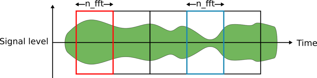
FFT takes a time-variant signal, and decomposes it in terms of discrete frequency components (frequency bins), with a magnitude and phase associated with each frequency component. Given a signal in the time-domain, which can be plotted as a function of time, we can decompose the signal using FFT and instead plot it as a function of frequency, where the number of frequency bins/length of the transform (n_fft) determines the granularity of the frequency. To apply the method on signals that vary in time, we usually first divide the signal into segments with n_fft number of samples.
Then, FFT is applied on each signal segment, and stacked in time.
This produces a waterfall display, which should be familiar from SDR applications or radios with frequency visualization capabilities.
This way of segmenting the signal in pieces that are decomposed using FFT gives us a waterfall diagram that has a concept of both frequency and time, which gives us the oppourtunity to pick out the frequency corresponding to the beacon signal. The resolution along the frequency axis is determined by n_fft, with a better resolution requiring a high n_fft, which divides the time-axis in larger segments and yields a lower time resolution in the final waterfall diagram.

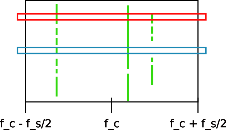
Regardless of n_fft, the frequency components go from –f_s/2 to f_s/2, where f_s is the sample frequency. In the drawing above, we’ve also included the center frequency, f_c. We’ll come back to that.
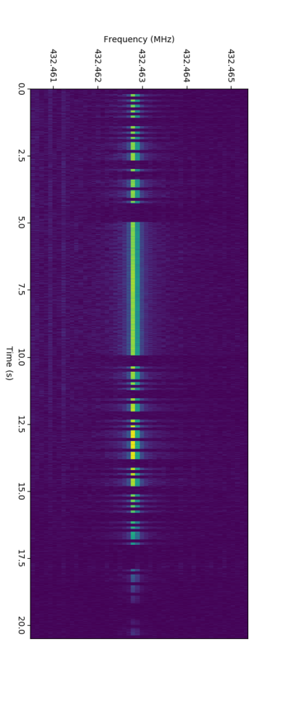
A more real example is the waterfall diagram of the beacon from the Extracting the antenna pattern from a beacon signal, pt. I: Initial investigations using autocorrelation, with n_fft = 1024 and sample rate 100 kHz.
LA1K’s beacons produce a single, clear tone which is turned on and off, which means that the signal should mostly be contained within specific frequency bins. During the very first blog posts (Preliminary measurements of the parabolic dish, Measurements of the parabolic dish in a free path environment, Using GNU Radio and Hamlib to calculate antenna diagrams), we picked the specific frequency bin by hand. This got to be a bit tedious, especially when changing the length of the transform, the frequency was changed or other parameters changed, so we wrote some code for picking the correct frequency bin automatically.
For an FFT with n_fft = 8, the frequency bins will be contained in 8 indexed bins.

Luckily, the correspondence between a given frequency bin in the Fourier transform and a frequency is simple to calculate in Python. Given an FFT of size n_fft, the relative frequencies are calculated through
relative_frequencies = np.fft.fftfreq(n_fft))

This gives us only the relative frequencies with respect to the given sample rate, where frequency 0 corresponds to the DC-component/a constant signal, and frequency 1 corresponds to the sample rate (and -1 to the negative sample rate). Converting these to actual frequencies in Hertz is them simply done by multiplying by the sample rate:
frequencies = relative_frequencies * f_s
Assuming samplerate of 1 MHz, we’ll just have the same numbers as above, only now in MHz.
In addition, FFT customarily returns an array over frequency bins, where the first position corresponds to the DC component, the n_fft/2-th position corresponds to half the sample rate, while the frequencies above corresponds to negative frequencies. If the FFT is taken over a signal consisting only of real numbers, the negative frequency components will just correspond to a mirror of the positive frequencies, since the concept of “negative frequencies” do not make much sense in the context of real signals. IQ samples are complex-valued, however, consisting of real and imaginary parts (or magnitude and phase), and actually do have a concept of negative frequencies (due to the phase part). We’d rather have the negative frequency components before the positive frequency components in order to have a meaningfully ordered frequency axis, which the function fftshift makes convenient for us.
frequencies = np.fft.fftshift(frequencies)

Now, the frequencies range from –f_s/2 to f_s/2, which correspond to the sample rate at which the data were acquired using the SDR. This still does not correspond to a real frequency in terms of actual radio waves. In order to get that interpretation, we need to go back to what the SDR actually does when it produces samples: The SDR tunes its local oscillator to a specific frequency, and takes samples relative to that frequency. This means that frequencies exactly at the local oscillator frequency correspond to a DC level, and that zero frequency in our FFT actually means the local oscillator frequency, or the center frequency. “Positive frequencies” are then frequencies with positive offset from the local oscillator frequency, while “negative frequencies” are frequencies with a negative offset from the local oscillator frequency. We therefore obtain the actual frequency axis in terms of the original radio signals by just adding the center frequency.
frequencies = frequencies + f_c

We can then translate frequency bins to actual frequencies, which we did in the previously displayed waterfall plot.
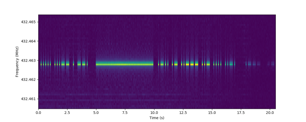
The beacon signal is clearly seen within the waterfall, but it is only mostly contained in a single frequency bin, it is also leaking a bit into the surrounding bins. The main reason for this is that the Fourier transform is made for decomposition of periodic signals, not time-variant signals like this. The Fourier transform decomposes a signal in terms of cosines, which have an extremely specific frequency and defines what it means to have a “frequency”. On the other hand, cosines have infinite extent, and can’t be localized in the time domain. Look at a cosine at a specific point in time, and it can’t be told apart from itself one, two or hundred periods later. We’ve decomposed our signal (finite in time, identifiable in time, multiple frequencies) in terms of cosines (infinite in time, very specific in frequency), which causes some weird effects. Some of these effects are seen above as leakage into other bins. In addition, the frequency of the beacon is not located exactly in the center of a frequency bin, meaning that two neighboring bins have large contributions from the signal.
In any case, the leakage is partly rectified by applying a windowing on the signal before the transform.
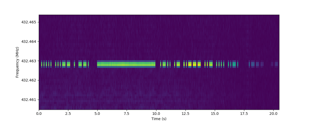
It looks nicer already, though it is still evident that two bins, and not only one have major contributions of the signal.
There are two alternatives here: Either pick the frequency bin that is closest to the frequency of interest, or interpolate. Both are rather easy to do:
Choosing the closest frequency bin:
bin_index = np.argmin(np.abs(frequencies - beacon_frequency))
signal_of_interest = fft[:, bin_index]
Interpolating:
from scipy.interpolate import interp1d
signal_of_interest = interp1d(frequencies, fft, kind='cubic')(beacon_frequency)
Turns out the latter works quite well for this type of signal.

Here, we’ve used cubic interpolation. The peak maximum of the interpolation corresponds well with the frequency of the beacon.
In some situations, especially when there is much noise, cubic interpolation might not be that appropriate and could produce unstable results. In that case we would be better off with just choosing the closest frequency bin.
After interpolating exactly at the frequency of interest, we have our beacon signal as a function of time.
![]()
The code for the frequency part of the analysis is given in frequency_analysis.py. Entry point can be interpolate_at_frequency(), which loads the IQ samples from a GNU Radio file, calculates the FFT, calculates the frequency axes for the FFT using the center frequency and sample frequency as obtained from the header file, and finally interpolates at the specified beacon frequency. This is done using load_and_calculate_spectrum(), which does all of that except for the interpolation part, instead giving the FFT throughout a specificed frequency range in terms of the original RF frequencies.
Pattern extraction
For the rest of the analysis, the plots, analysis steps and corresponding motivations have mostly been given before in the two previous blog posts (Extraction of the antenna pattern (…) pt. I (…), pt. II), but we’ll reiterate a bit here. The code for the pattern extraction is given in cw_extraction.py, and the main entry point function for signal level extraction is given as extract_signal_level_from_periodic_cw_signal().
The first, most integral part is to apply autocorrelation to the signal in order to extract the signal periods. This is simply done by running np.correlate(signal, signal, 'full'), which returns the autocorrelation from -len(signal)-1 to len(signal). Appropriate preprocessing should be run before this, which is done in our module by taking the logarithm and subtracting the moving average for an appropriate window size.
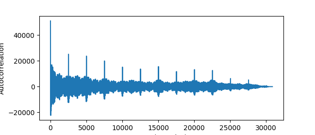
This yields an autocorrelation diagram, as seen before. The peaks are used to estimate the signal period. Since the first peak at a non-zero lag usually is quite clear and usually is larger than the other peaks, we sort the correlation values and select the first which appears after a lag of more than 1 second in order to skip over the peak at lag = 0:
signal_period = int(sorted_correlations[sorted_correlations > peak_thresh][0] )
We’ve probably been too lucky with our signals in that there are no larger peaks, but in the worst case is a later peak chosen and more than one signal sequence is included in the found signal period.
Here, we could also have checked at each integer multiple of the signal period and checked to see whether there is a larger peak in the local area. If there are shifts between the sequences or noise, these will be propagated into shifts in the autocorrelation peaks. These could be used to improve the overall estimate by averaging, however, the peaks will also get less prominent at the larger lags. The first peak will probably represent a good average, as this finds the best shift that compares the full signal at the first lag, while the rest of the peaks only represent a subset of the signal.
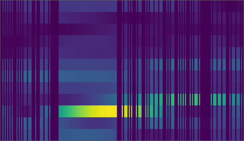
Then, the signal is divided in segments according to the found signal period:
num_segments = len(signal_periods)
segment_image = np.zeros((num_segments, signal_period))
segment_counter = 0
for i in np.arange(0, num_segments):
    sequence = samples[i*signal_period:(i+1)*signal_period]
    segment_image[i,0:len(sequence)] = sequence
segment_image produces the image we’ve seen before:
The autocorrelation and signal segmenting is done in divide_periodic_cw_signal_in_segments().
In the previous blog post, we found that it was necessary to cross-correlate each sequence against the first in order to correct for individual shifts and possible timing problems. We do this in rectify_sequences_by_crosscorrelation(). np.correlate() is again used to calculate correlation, after appropriate preconditioning of the signal, and each signal sequence is rectified.
We can then construct a signal template matching the high and low parts of the signal, done in construct_signal_template(). The rectified sequences are used to calculate a preliminary signal threshold:
sequence_template = np.max(segment_image_rectified, axis=0) > np.mean(segment_image_rectified)
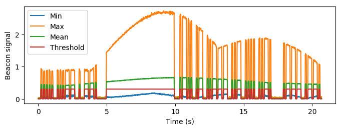
As discovered the last time, this does not necessarily match the signal that well as hoped. We therefore found it necessary to do some ad-hoc adjustments to it by calculating a local signal threshold for each sequence based on the original sequence template. Having done this, we produce a large template for the entire signal which can be used for thresholding.
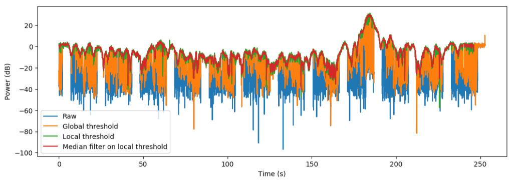
Using the full template, we can threshold the signal and remove some rising samples at the edges using median filtering:
from scipy.signal import medfilt
power_db = 10*np.log10(medfilt(samples[template > 0])**2)
Finally, we can plot the antenna diagram using the procedures as outlined in a Using GNU Radio and hamlib to calculate antenna diagrams.

To use the presented modules for this, we’d first have to measure IQ samples using GNU Radio, saving to GNU Radio file meta sink filenames e.g. iq_samples.dat and iq_samples.dat.hdr (GRC flowgraph example), and simultaneously measuring azimuth angles of the rotor using rotctld_angle_printer.py to e.g. angles.dat while the rotor is rotating.
Firing up Python, we can load the rotor angle measurements:
from antenna_pattern.combine_samples_and_angles import load_angles, interpolate_angles
angles = comb.load_angles('angles.dat')
Then we can use the presented procedures to extract the signal level from the periodic morse signal:
from antenna_pattern.cw_extraction import extract_signal_level_from_periodic_cw_signal
timestamps, signal_level = extract_signal_level_from_periodic_cw_signal(filename='iq_samples.dat', frequency=1296963000.0)
Using the extracted timestamps, we can interpolate the azimuth angles:
azimuth = interpolate_angles(timestamps, angles)
This can then be plotted in a polar diagram using e.g.
import matplotlib.pyplot as plt
plt.polar(azimuth*np.pi/180.0, np.log10(signal_level))
, probably with some extra signal level shifting and dB handling as outlined in Using GNU Radio and hamlib to calculate antenna diagrams.
We now have a usable procedure for estimating antenna patterns using our beacons only, which we’ll probably have some use for in the future for checking antenna properties in the wild, with less hassle than we had to do in Rough antenna pattern measurements using a local radio beacon. We’ll also come back to a more probabilistic approach over the autocorrelation approach, but this is more for the fun of it and not out of necessity. 8)
Previous and future parts of the series:
- Extracting the antenna pattern from a beacon signal, pt. I: Initial investigations using autocorrelation
- Extracting the antenna pattern from a beacon signal, pt. II: Measurements of LA2SHF
- Extracting the antenna pattern from a beacon signal, pt. III: Frequency analysis and code (current post)
- Extracting the antenna pattern from a beacon signal, pt. IV: Probabilistic approach

0 Comments
2 Pingbacks