
As a part of earlier blog posts ([1], [2]), we developed a couple of tools for measuring antenna patterns against remote beacons. We outline the usage of these tools in this blog post.
While in our case specifically tailored against measuring antenna patterns, the functions we have developed can also be useful in a wider setting, as we also provide e.g. concise functionality for reading GNU Radio-produced files into Python for offline/non-live analysis, without having to re-run the file in a GNU Radio flowgraph. To our knowledge, clear information about how to do that is not very available :-). It also serves as a nice example on the utilization of both GNU Radio and hamlib to solve a simple practical problem.
The main problem at hand is how to measure the power of an antenna at various azimuth degrees by setting up a constant signal source, rotating the antenna and continuously measuring the reception power. Signals that are turned on and off (i.e. CW beacons) can also be used, but the code here mainly assumes that the signal is constant. Some pre-processing will be necessary for other kinds of signals.
The main motivation is to characterize directive antennas, for debugging purposes or for evaluating their performance when antenna chambers are not available. This could be done manually, but this is a tedious and error-prone procedure and is preferably automatized.
The toolset consist of a couple of scripts:
- Script for continuous read-out of rotor angles from rotctld, printing only when angles differ
- GRC scripts for continuous recording of IQ samples (or a subset of log power samples) from an SDR using GNU Radio
- A Python module for reading in the GNU Radio samples from file, the angles from file and for combining them and doing post-processing to produce azimuth-resolved power for antenna diagrams. This includes functionality for reading GNU Radio metafiles, as produced from a GNU Radio file meta source.
Record angles from rotctld
We use rotctld to control all our rotor controllers. Reading out the current angle is then a simple matter of connecting to a socket,
rotctl = socket.socket(socket.AF_INET, socket.SOCK_STREAM)
rotctl.connect((rotctld_host, rotctld_port))
and then repeatedly ask for the current angle:
rotctl.send(b'p\n')
azimuth, elevation = rotctl.recv(1024).decode('ascii').splitlines()
In our script, we print the current timestamp and angles to stdout if the current angle differ from the previous angle. This way, we can keep only the relevant information down to the precision of the rotor controller. Example output:
timestamp                  azimuth    elevation
2018-02-17T15:49:55.395318 270.000000 -5.000000
2018-02-17T15:49:59.486617 269.900024 -5.000000
2018-02-17T15:49:59.540253 269.799988 -5.000000
2018-02-17T15:49:59.611497 269.700012 -5.000000
2018-02-17T15:49:59.664928 269.599976 -5.000000
2018-02-17T15:49:59.736160 269.500000 -5.000000
2018-02-17T15:49:59.789507 269.400024 -5.000000
2018-02-17T15:49:59.860668 269.299988 -5.000000
2018-02-17T15:49:59.985031 269.200012 -5.000000
While turning the rotor, we then have a complete log over where the rotor is at a given time. The datatable can easily be read using e.g. pandas. A wrapper can be found here.
Collecting IQ samples (or the power spectrum) in GNU Radio
We need to collect IQ samples from GNU Radio while turning the rotor, for later processing into power estimates.
Finished. 8)
Adding a GUI frequency sink for visual feedback is probably also a good idea, in order to catch any errors during operation.
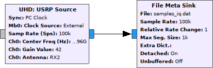
The above GNU Radio flowgraph collects IQ samples to a GNU Radio metafile “samples_iq.dat” at center frequency 1.29696 GHz with a bandwidth of 100kHz. This was suitable for us to record our beacon, but the frequency will have to be tuned for other applications. The file meta sink will contain enough information for GNU Radio to reproduce the data stream offline, complete with timestamps – and also be enough for us to do offline analysis and interpolate the samples against the recorded azimuth angles. Having raw IQ samples enables for offline experimentation, which was very useful for us.
(We had to record the files using “Detached header”. Having the header as a part of the datafile seemed to produce corrupt files in our case, for some reason.)
Collecting all IQ-samples can produce rather large files. We’ve limited the samplerate somewhat, reducing the file size to approximately 200 MB for a full turn of the satellite dish rotor. If we need to collect samples for a longer time, it can be desired to reduce down to exactly what we need by calculating the power spectrum in GNU Radio itself, and outputting only the frequency bins of interest. The flowgraph below does this:
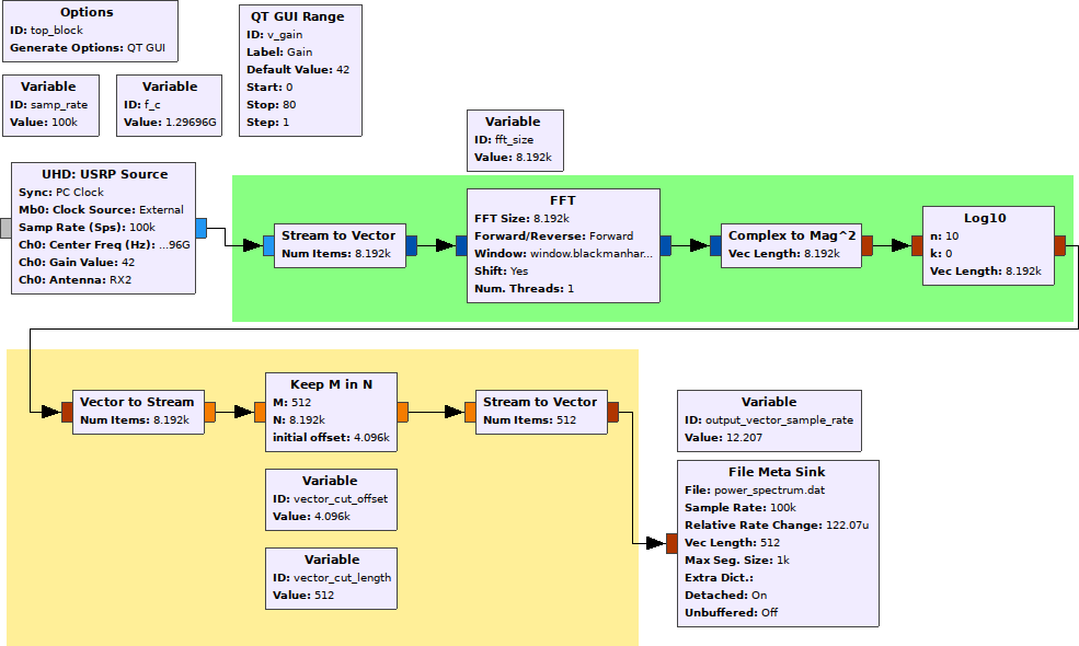
The first (green) part calculates the discrete fourier transform of the input data, and then takes 20*log10(abs(...)) of the frequency bins. This produces the power spectrum, resolved as a stream of vectors, where each vector corresponds to a power spectrum frame for a given time instant.
In our case, we were interested only in a specific frequency bin, corresponding to the frequency of the beacon we were measuring. We could therefore discard most of the frequency bins. The vector stream is converted back to a normal datastream, and we keep (in this case) 512 of the frequency bins (vector_cut_length), at an appropriate offset (vector_cut_offset). We could here also have modified the offset and length to produce only the frequency bin of interest. The process is illustrated beneath:
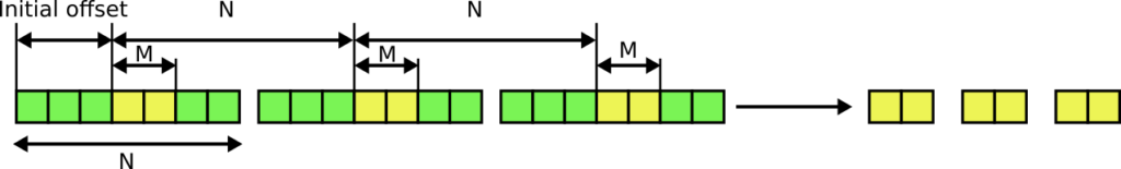
Using the “keep M in N”-block to extract specific vector indices from a vector stream.
In the blog posts, we chose not to use this approach, but rather calculated the power spectrum offline from the IQ samples. This part is still included for interest, especially as this part was present in the screenshot displayed in an earlier blog post.
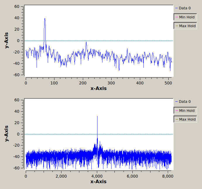
Running the power estimation GRC script against a signal source: The full spectrum on bottom, the subset spectrum on top.
We also make sure to calculate the correct rate change for the file meta sink, since the sample rate for the vectors in the vector stream will be different from the sample rate of the individual samples. This will ensure that the rx_rate tag in the output file will correspond to the rate of the vector elements, and not each individual sample, which makes life slightly easier in the off-line analysis end.
Loading GNU Radio files in Python
It turns out that the metafile file format is rather simple, as long as the file is written with a detached header (the header in a separate file). The file will consist of a long binary stream of individual samples in the given dataformat. The IQ samples will, for example, be output to file as a long stream of complex numbers, the first number corresponding to the first sample, the second number to the second acquired sample, etc, which can be read back into an array quite easily.
Example for the IQ samples:
import numpy as np
samples = np.fromfile(‘samples_iq.dat’, dtype=np.complex64)
This will be a one-dimensional array containing complex values, each array position corresponding to a sample as acquired from the USRP source.
For the log power spectrum data that is written to ‘power_spectrum.dat’, they could be read using:
samples = np.fromfile(‘power_spectrum.dat’, dtype=np.float32)
Since the power spectrum data actually are in vector format here, the array needs to be reshaped to a matrix in order to be interpreted correctly:
samples = np.reshape(samples, (-1, vector_length))
The header file also contains some valuable information. Luckily, GNU Radio has functionality for parsing this into handy structures, which is exposed as the Python module gnuradio.blocks.parse_file_metadata. The essential information here is the datatype (complex, float, …), the item size (from which we can calculate the vector length, if the stream is a vector stream), and tags. The most important tags for us will be rx_time and rx_rate, which correspond to the timestamp of the first received sample and the sample rate of the stream, respectively. We use these to calculate timestamps for each GNU Radio sample.
In our Python module, we have functionality for reading the metafile header (load_gnuradio_header(), see here for implementation), and for loading the samples (load_gnuradio_samples(), see here for implementation). The sample loading function handles both vector and normal streams, and calculates timestamps for each sample or vector frame using the rate and first timestamp. We currently handle only complex double and float datatypes, and we don’t handle rate changes, assuming constant data rates. The files are mapped as memory maps instead of being read directly into memory. This can be convenient for very large files.
Calculating the power spectrum from IQ samples in Python
Given that we did not calculate the power spectrum in GNU Radio, we must compute it using the IQ samples somewhere else. In Python, this is easily done using numpy:
fft_res = np.fft.fftshift(np.fft.fft(iq_samples[i*n_fft:(i+1)*n_fft]))
spectrum[i,:] = 10*np.log10(np.abs(fft_res[start_bin:end_bin])**2)
We divide the IQ samples in frames, take the (shifted) Fourier transform of each frame, and take the log power magnitude of each Fourier frame. Here, we also take a subset of the frequency bins. This was a bit memory intensive, so we had to discard frequency bins we did not have any use for.
This part is implemented in the power_spectrum() function (see here for implementation). We also calculate new timestamps for each frame from the original sample timestamps, assuming constant data rates, so that each FFT frame is ready for interpolation against the recorded rotctld angles.
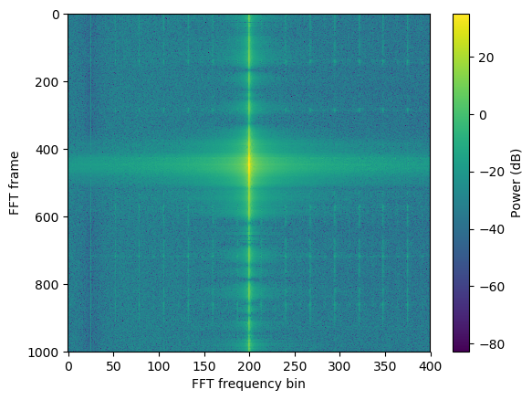
FFT power spectrum example. The strongest signal at frequency bin 200 corresponds to the beacon which was measured, and is the signal which is plotted against the azimuth angle below.
Interpolating angles against the samples and plotting the power in polar diagrams
We now have (the subset of) a power spectrum, corresponding timestamps, and recorded angles and timestamps. To get e.g. azimuth angles for each power spectrum frame, we interpolate.
interpolator = scipy.interpolate.interp1d(azimuth_timestamps, azimuth)
interpolated_azimuth = interpolator(power_spectrum_timestamps)
This is essentially it, but we also do some massaging to make both datasets use the same timeframe, and ensure correct angles when the rotor has stopped. We support both azimuth and elevation interpolation. The interpolation is in the function interpolate_angles() (see here for implementation), which takes in the angles and timestamps as read from the rotctld log file and timestamps as obtained from load_gnuradio_samples() or power_spectrum() to produce a final interpolated azimuth (or elevation) angle.
Complete example:
import combine_samples_and_angles as comb
angles = comb.load_angles('angles.dat')
timestamps, iq_samples = comb.load_gnuradio_samples('iq_samples.dat')
spectrum_timestamps, power_spectrum = comb.power_spectrum(timestamps, iq_samples)
azimuth = interpolate_angles(spectrum_timestamps, angles, 'azimuth')
Let’s say that frequency bin number 200 in the power spectrum contains a strong beacon that we want to use. The power of interest is then
power = power_spectrum[:, 200]
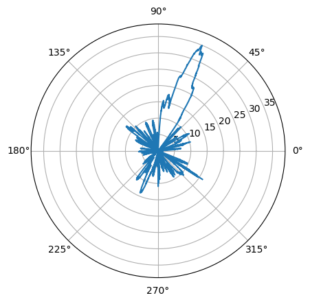
After having done the above steps, we can produce an antenna diagram quite simply:
plt.polar(azimuth*np.pi/180.0, power)
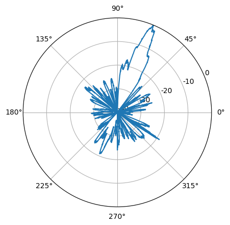
However, since the power here is calculated without a real reference, and since there will be arbitrary negative values which the polar diagram can’t handle, we have to do some additional steps in order to get something which can be interpreted. It is customary, for example, to let the maximum power have value 0 dB, and let the rest of the distribution take negative values from there and down. The lower limit of the polar diagram should be -40 dB. We achieve this by manipulating the power array a bit and changing the axis values:
min_power = -40
power = power - np.max(power) - min_power
power[power < 0] = 0
ax = plt.subplot(111, projection='polar')
plt.plot(azimuth*np.pi/180.0, power)
We now have the power, but with apparent values from 0 to 40. We need to flip the axis labels a bit in order to make it start at -40 dB and end at 0 dB. We also add circles at every 5 dB increment:
ax.set_rmax(-min_power)
ax.set_rmin(0)
ticks = np.linspace(0, -min_power, 5).astype(int)
ax.set_rticks(ticks)
ax.set_yticklabels(-1*np.flip(ticks, -1))
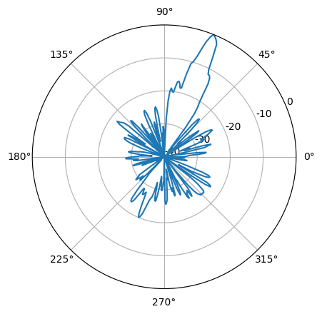
We could in addition also have taken the mean over angles less than the time resolution in order to improve the antenna diagram statistics, and make it be less noisy.
We first reduce the azimuth down to our desired resolution:
azimuth = np.round(azimuth)
The azimuth angle and power estimates are then combined in the same pandas dataframe:
import pandas as pd
df = pd.DataFrame({'azi': azimuth, 'power': power})
Finally, we group the dataframe rows by unique azimuth angles and take the mean over each group:
power = df.groupby('azi').mean().power.as_matrix()
azimuth = np.unique(azimuth)
plt.polar(azimuth*np.pi/180.0, power)
The presented code (except for the last snippets) is all available on GitHub. We hope it might be useful for someone.


0 Comments
1 Pingback