Plotting spotting calls on a map

LA3WUA Øyvind came to me late Monday evening last week, desperate, wanting a map to visualize the calls which had spotted our 4m beacon, LA2VHF/4. No problem, Øyvind. 8). Here is also a post describing how it can be done, so that you can do it yourself the next time.

The problem at hand is to visualize contacts that have spotted our beacon on a map in order to visualize propagation. The solution here can be considered a follow-up to an earlier blog post, Plotting Norwegian ham radio contacts on a map using Pandas, Cartopy and Geopy, where we plotted Norwegian calls on a map over Norway. In the current post, this is extended to European contacts.

LA3WUA had already provided for me an ADIF file containing the calls and the corresponding locators, which he had meticulously looked up from QRZ.com. Locators or coordinates for a given call are usually not that easily available, and will in general have to be looked up from clublog or similar. The coordinates from clublog will probably not be accurate for more than the country in question, while the coordinates LA3WUA had looked up will be as accurate as the user at QRZ.com has made them.

An ADIF parser for Python was hacked together based on rough regular expressions (more on that in a later blog post, probably) to yield a pandas dataframe containing the calls:

  call   date     filename      time gridsquare
0 DL9DAC 20180601 contacts.adif 1948 JO31qi
1 OM3CLS 20180601 contacts.adif 1944 JN99fc
2 GD3YEO 20180601 contacts.adif 1940 IO74rd
3 ON4KST 20180601 contacts.adif 1750 JO20hi
4 DH5YM  20180601 contacts.adif 1711 JO60rd
5 HA1VHF 20180601 contacts.adif 2045 JN87gf

The next step was to convert locator to latitude/longitude coordinates. The letters in the locators are converted to the corresponding alphabet number (i.e. A -> 0, B -> 1, …) while the numbers are taken directly. The characters at the first, third and fifth position are combined to yield the longitude, while the others are combined to yield the latitude.

Here is Python code for converting a maidenhead locator string to latitude/longitude coordinates:

def locator_to_latlon(locator):
    squares = np.zeros(6)

    for i in range(0, np.min(len(squares), len(locator))):
        if locator[i].isalpha():
            squares[i] = ord(locator[i].upper()) - ord('A')
        else:
            squares[i] = int(locator[i])

    longitude = squares[0]*20.0 + squares[2]*2.0 + (squares[4]+0.5)/12.0 - 180.0
    latitude = squares[1]*10.0 + squares[3]*1.0 + (squares[5]+0.5)/24.0 - 90.0

    return latitude, longitude

The longitude and latitudes are then extracted from the locators using

spots['latitude'] = spots.apply(lambda row: locator_to_latlon(row.gridsquare)[0], axis=1)
spots['longitude'] = spots.apply(lambda row: locator_to_latlon(row.gridsquare)[1], axis=1)

, yielding

  call   gridsquare latitude   longitude
0 DL9DAC JO31qi     51.354167  7.375000
1 OM3CLS JN99fc     49.104167  18.458333
2 GD3YEO IO74rd     54.145833  -4.541667
3 ON4KST JO20hi     50.354167  4.625000
4 DH5YM  JO60rd     50.145833  13.458333
5 HA1VHF JN87gf     47.229167  16.541667

We obtain our own location using

la1k_lat, la1k_lon = locator_to_latlon('JP53ek')

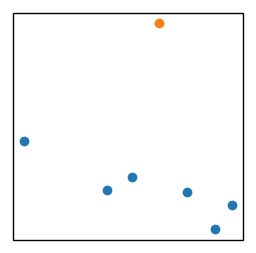
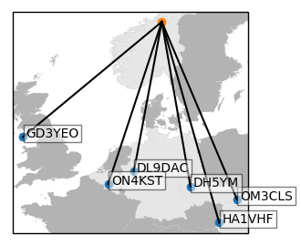
Plotting these coordinates on a map can then be done using

import matplotlib.pyplot as plt
import cartopy.crs as ccrs
plt.clf()
projection = ccrs.LambertConformal()
ax = plt.axes(projection=projection, aspect='auto')

ax.plot(spots.longitude, spots.latitude, 'o')
ax.plot(la1k_lon, la1k_lat, 'o')

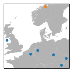
We are missing countries, however. Like in the earlier blogpost, we’ll do this using natural earth shapefiles in cartopy.

import cartopy.io.shapereader as shpreader
reader = shpreader.Reader(shpreader.natural_earth(resolution='10m', category='cultural', name='admin_0_countries'))
ax.add_geometries(list(reader.geometries()), projection, facecolor=(0.7, 0.7, 0.7))

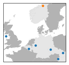
We also wanted to highlight the countries. The country names can be reverse-looked up from the coordinates using geopy:

from geopy.geocoders import Nominatim
geocoder = Nominatim()
spots["geocoder_res"] = spots.apply(lambda x: geocoder.reverse([x.latitude, x.longitude], language='en'), axis=1)

(language='en' is important, otherwise the country names will be in the local language of the country in question. Natural earth shapefiles don’t have entries for Deutschland or Magyarország, unfortunately, only Germany and Hungary.)

The country name is extracted using

spots['country'] = spots.apply(lambda x: x.geocoder_res.raw['address']['country'], axis=1)

This will yield

  call   country
0 DL9DAC Germany
1 OM3CLS Slovakia
2 GD3YEO Isle of Man
3 ON4KST Belgium
4 DH5YM  Czechia
5 HA1VHF Hungary

We take the countries out and add Norway

desired_countries = spots.country.unique()
desired_countries = np.append(desired_countries, 'Norway')

and then go through the map shapes to find the corresponding country names (GEOUNIT in the natural earth shapefile structure):

plot_countries = []

for country in list(reader.records()):
    if country.attributes['GEOUNIT'] in str(desired_countries):
        plot_countries.append(country.geometry)

ax.add_geometries(plot_countries, projection, facecolor=(0.9, 0.9, 0.9))

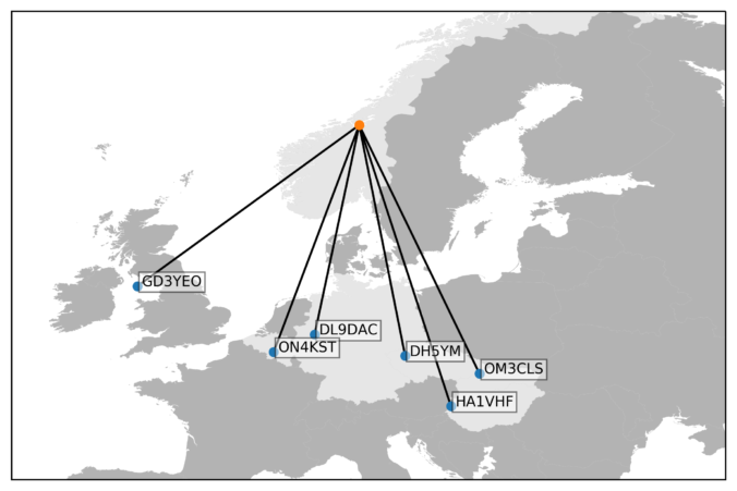
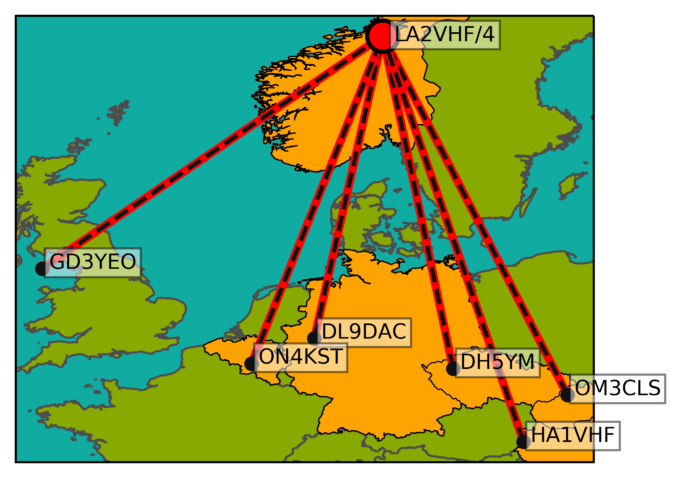
In the blog post, we plotted lines from our location to each spotter’s location, and added text blobs with the callsigns.

for index, spot in spots.iterrows():
    ax.text(spot.longitude+0.3, spot.latitude, spot.call,
    bbox={'facecolor':'white', 'alpha':0.5, 'pad':2})
    ax.plot([spot.longitude, la1k_lon], [spot.latitude, la1k_lat], color='black')

We also went a little overboard with the colors, in order to make the map scream at the reader with enforced jolliness.

The sea color was applied by ax.background_patch.set_facecolor(sea_color), while the colors elsewhere were supplied using the facecolor and edgecolor keywords to the add_geometries() function when plotting the countries. The colors were selected by applying a diseased brain to the problem of selecting colors.

We’ll probably come back to more map fun in a later post. We have some plans for live plotting of logged contacts and DX cluster spots.