In the first blog post of this series, we analyzed the beacon signal from LA2VHF to obtain the enveloping, azimuth-dependent variation in reception power. This was something we needed in order to be able to estimate the antenna diagram against our beacons.
LA2VHF sends out a morse sequence which repeats itself at regular intervals. By applying autocorrelation to the signal, we were able to extract the period of the morse signal. We used this to segment the signal into its constituent morse sequences. The sequences were then used to nicely threshold the signal, and we could interpolate over the gaps to yield the azimuth-resolved signal level.

LA2VHF is a 2 m beacon, however, and this was measured using the parabolic dish on its 23 cm antenna. For today’s blog post, we wanted to show the same approach on LA2SHF, our 23 cm beacon.
As it turns out, measuring a signal source which transmit on the actual wavelength for which our antenna was built, in an amplifying parabolic dish, causes the approach above to completely break down. The lobe corresponding to the line of sight against the beacon will dominate over the rest of the signal.
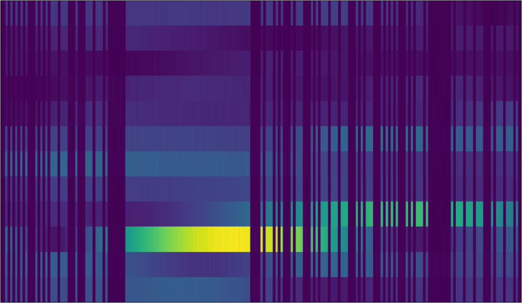
Here is the signal level from LA2SHF, our 23cm beacon, as a function of time as we sweep the rotor over all azimuth angles:
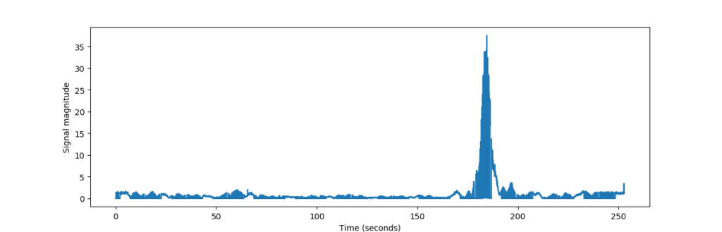
We can plainly see the main lobe with an abnormally high signal level compared to LA2VHF, and the rest being comparably suppressed on a linear scale. During the measurement, we actually had to reduce the gain in order to make the beacon not completely saturate the receiver. This is actually good, this means that our system is working very well on the wavelengths for which it was meant: but it causes an endless stream of trouble for our rather naive analysis.
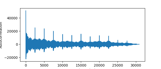
Taking the autocorrelation of this signal will mainly show how this large lobe is correlated with the rest of the signal:

There are some very small peaks that indicate the morse sequence, but the behavior here is mostly due to the pattern itself.
Luckily, however, there is a quick solution to this – take the logarithm. This is actually what we’d do in any case, as we’d rather work on dB scale when it comes to power estimates.
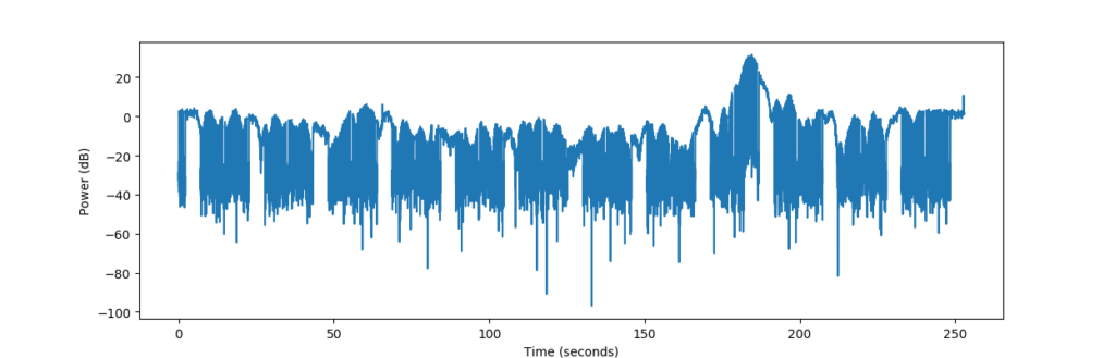
Having taken the logarithm of the signal, the lobes throughout the signal are more comparable against each other, and the main lobe no longer dominates over the rest. This also enhances the noise in the gaps of the signal, which would normally be problematic – but is actually handled very well by the autocorrelation.
This is almost like the situation we had for LA2VHF. The peaks corresponding to the morse sequence are very clear, and will be easy to extract, and the signal is no longer dominated by the modulating behavior. Probably, the noise did not affect the autocorrelation that much since the noise mostly is uncorrelated.
Once the extracted signal period is used to divide the signal into sequences, it turns out that there are more obstacles. For LA2VHF, we had the following sequence image:
The sequences were here extremely well aligned, no problems. For the measurements of LA2SHF, the situation is far worse:

The sequences are only approximately aligned. Zooming in further:
This is slightly problematic, as we in previous week’s approach segmented the morse signal based on the mean and maximum along all sequences, and blindly applied this signal template to each sequential part of the signal. There, we got good results since all sequences were perfectly aligned. If we were to do that here, we would misclassify background as signal and vice versa, and post-process the signal to become even worse than the raw signal.
Symptoms of this behaviour is available in the autocorrelation data. For LA2VHF, the peaks were in the previous week’s blog post placed exactly at a regular interval of 2020 samples, while for LA2SHF the peaks are more irregularly placed. Unfortunately, the full autocorrelation does not give any information of how much each sequence is offset with respect to each other, as the autocorrelation correlates the full signal without being aware of sub-sequences. We are now aware of subsequences, however, and can use a similar technique, cross-correlation, to investigate in more detail the offset of one sequence with respect to the next.
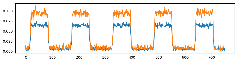
The first part of two sequences that are offset approximately 2 samples with respect to each other is shown below:
Taking the crosscorrelation of the two sequences will systematically shift the first sequence at various lags and correlate it against the second sequence. This is similar to autocorrelation, except that the lagged signal is another signal instead of the signal itself, and the largest peak will typically not be positioned at x = 0.
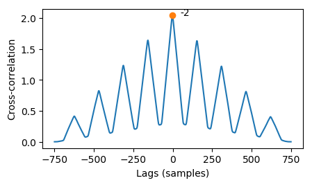
The cross-correlation produces peaks where the lagged copy of the first signal is similar to the second signal. If the signals actually are lagged copies of each other, the first peak will usually appear at the lag. The lag (-2 samples) can then be used to match the signals perfectly in time:
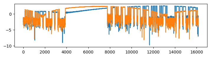
This was very clear for this short timespan, but again: The azimuth-dependent modulation will dominate over the sequencing behavior, and again cause trouble.
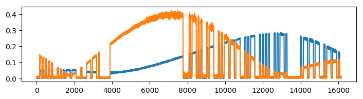
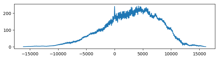
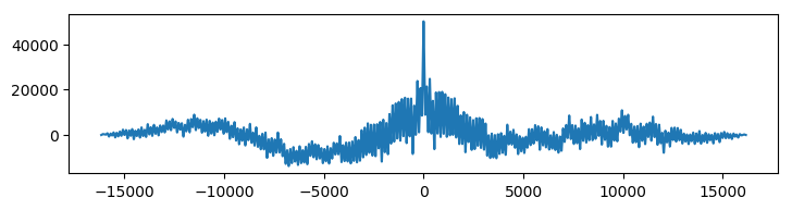
Here, taking the cross-correlation will probably just find the lag at which the large lobe in the orange signal matches with the large lobe of the blue signal, and this behaviour will dominate over the inherent shift in the morse sequence. The crosscorrelation below shows a large peak at where we expect the morse shift to be, but there is also a large, broad peak at 5000 samples, which indicates the lag of the lobes.
Again it turns out that just taking the logarithm actually makes the sequences comparable enough to yield a more clear correlation function. For good measure, we’ve also removed the mean.
Good enough for us! Still, this might not hold in general, so be careful.
Autocorrelation of the original signal has given us the rough behaviour of the sequencing and given us where to cut the signal into sequences, and cross-correlation can technically find the offset of each sequence with respect to the others if there are deviations in the autocorrelation peaks. So far, the analysis has not become that much more hairy. Everything will be fine! We’ll have a blog post on Wednesday. The author can sleep well.
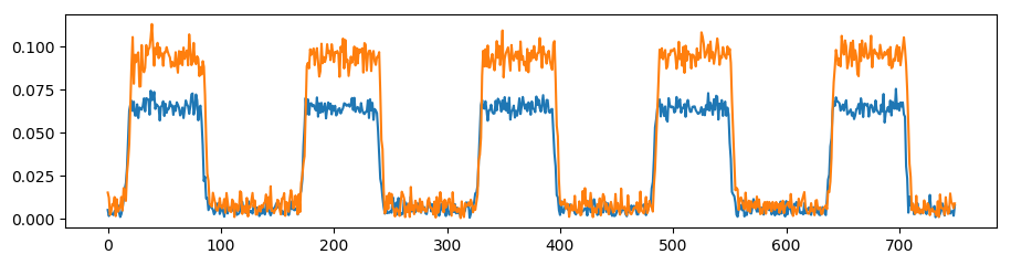
This was where I discovered that it was not actually possible to find the exact offset by cross-correlation, as it seems that the offset varies throughout each sequence.
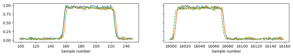
The plot above shows two normalized sequences from two points in time along the sequence. Blue and orange are the original sequences, while green dotted signal is the orange being attempted matched with the blue sequence. For the first part of the sequences, samples 100-240, the sequences are reasonably well matched if the orange sequence is shifted 2 samples to the left. But later on in the sequence, the orange sequence is actually already well matched with the blue sequence, and moving it 2 samples to the left will actually make it mismatch. The timing is actually not consistent throughout the entire signal. We’ve been had!
Plotting the sequences in an image confirms this trend. The first sequence, for example, is shifted to the left with respect to the next sequence for the first 150 samples, but after 2325 samples, it is actually slightly shifted to the right. The same behavior can be seen for the other sequences.
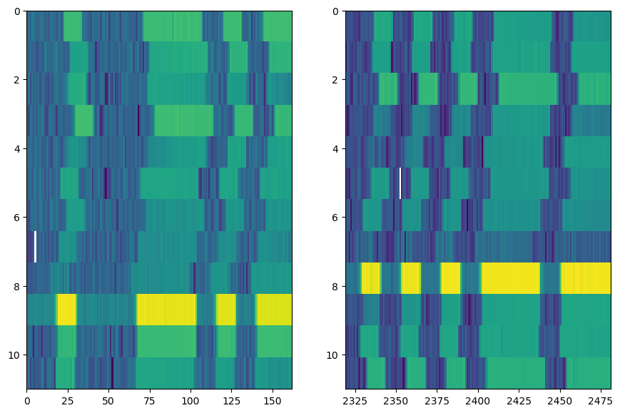
This is not a consistent behavior that is actually possible to entirely rectify for using crosscorrelation, unless we were to divide the signal further into smaller blocks along each sequence.
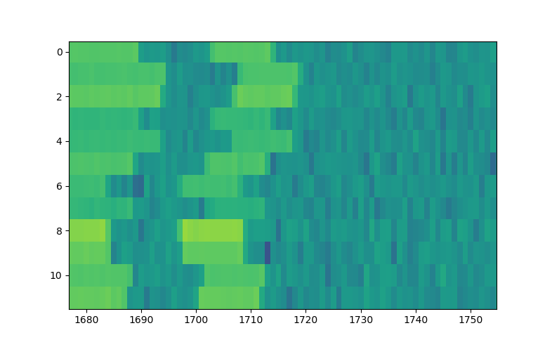
We can see quite clearly where the sequence seems to shift in a weird way: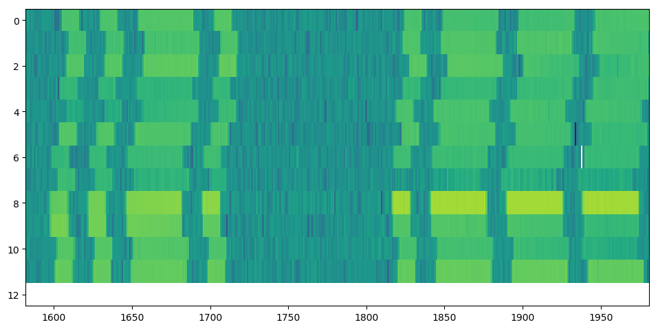
Before the gap from approximately 1720 to 1810 samples, the sequences are shifted in a specific direction with respect to the next sequence, but are shifted the other way after the gap. There might be multiple reasons for this behaviour. It could be actual timing problems in LA2SHF. Or, more likely: It could just be problems with timing during the reception. LA2SHF was acquired at a far higher samplerate (1 MHz vs 1 kHz) than LA2VHF last week, and it might be that the computer or the USRP for some reason was not able to handle the samplerate that well. Otherwise, it could also be that timing problems are present in both LA2SHF and LA2VHF, but are more noticable here due to the high samplerates. We’ll look more into this at a later point, but for now we’ll just try to make do with what we have.
Applying cross-correlation to each sequence isn’t going to fix the timing, but it will partially fix it: 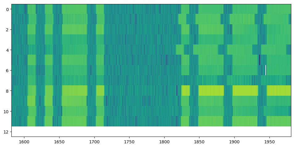
The cross-correlation will find the lag that mostly matches the signal, and while there will be some places where they do not match, the signal in its entirety will be mostly matched. We’ll therefore avoid matching at subsequence level, and just match each sequence against each other for now.

We have to add some ad-hoc processing to deal with the problems caused by this, however. After having approximately matched the sequences and found the signal template, matching the signal template against each sequence in the raw signal will still cause misclassification. We’ll deal with this with some thresholding applied to each individual sequence.
We first decide that misclassifying a background sample as a signal sample is a very serious offence, while misclassifying a signal sample as a background sample is not that serious as it will just be interpolated instead of being included in the pattern directly. A mis-classified background sample will on the other hand make the pattern look bad.
This is fine, for example:

Here, the original signal template would include a large part of the background. We’ve rectified the signal template by thresholding the signal locally for this specific sequence, and were able to reduce the template to the actual signal parts. The fact that one sample in the long BEEEP is misclassified as background is fine, as argued above.
The local thresholding is a bit involved. Part of the problem with thresholding is that the signal amplitude varies throughout the sequence due to the azimuth-dependent modulation. By using the signal template, we could guess at where the signal is high and low, and use moving average to do a rough estimate on the modulated signal level. We can then use the moving average to normalize the signal:
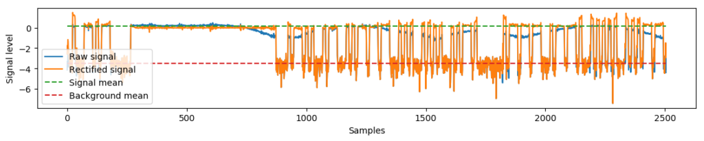
Here, the signal goes from varying up and down in level to being a bit more uniform. One additional plus point is that we already have samples that have been thresholded as belonging to the background according to the signal template, and we can ignore them in the normalization. This makes the separation distance much higher. In the plot above, we’ve also estimated the mean background level and mean signal level from the templated, normalized samples, which we can use to create a better threshold. Keeping samples already classified as background as background, we can then threshold misclassified background samples back to the background, and tailor the morse template for this specific sequence.
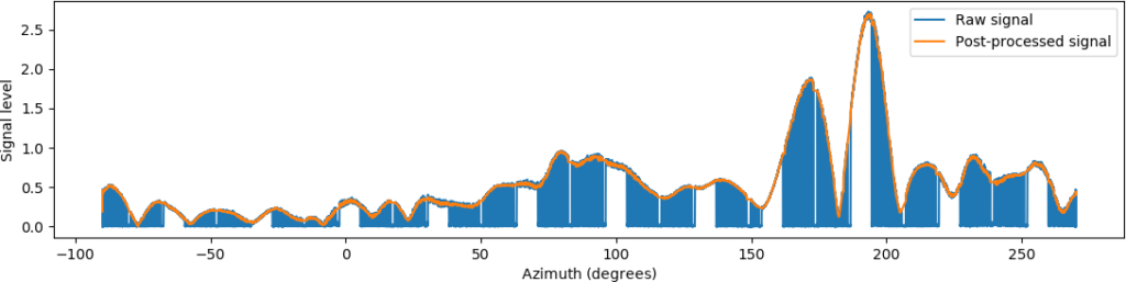
Below are shown the various iterations of the method:
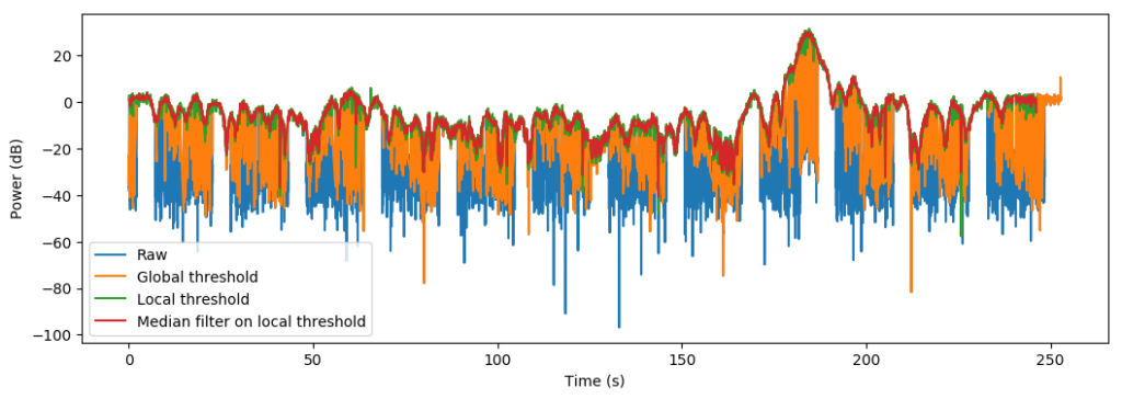
The global threshold is with classification of samples as signal according to the signal template as matched against each sequence, where matching offset has been found through the cross-correlation earlier. This pattern is still as bad/worse as the raw pattern since there is misclassification of background samples. The local threshold is the classification of the signal after the template has been tailored against each sequence. Finally, a median filter is applied to produce the final result.
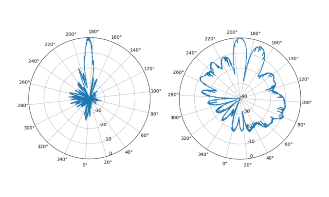
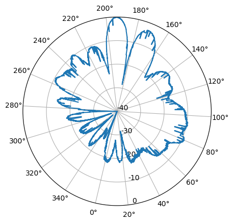
Plotting this in a polar diagram produces a nice result:

We can also apply a mean to improve the pattern a bit.
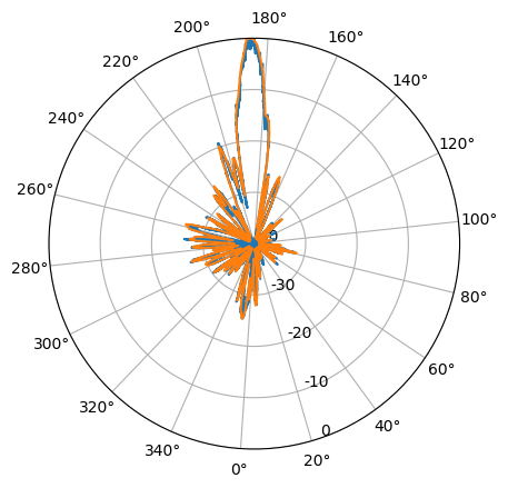
Finally, the ad-hoc approaches here made to rectify for the timing offsets are robust enough to also work well enough for the already timed and comparable LA2VHF measurement:
This pattern has some stripes placed here and there, which is due to suboptimal interpolation over gaps with rising samples. This antenna diagram shows suboptimal, less directive behaviour, which is expected as LA2VHF is well outside the range of the antenna in use.
The experiences with LA2SHF shows the problems with the correlation approach, as the timing and overlapping needs to be very accurate in order for it to work well. It doesn’t work that well when the timing is more arbitrary or has jitter, and we have to employ less elegant ad-hoc solutions. The probabilistic approach, to be presented at a later stage, might actually have some merit in this case. A combination of a correlation-based approach and a probabilistic approach will probably yield the best results.
As for the timing problems, we’ll either get back to it or figure out that we’ve made a stupid mistake and update this post in silence. Stay tuned! Or don’t! For the next blog post in this series, we’ll go more into some frequency analysis details used to actually obtain the beacon signal, and publish and go through the code so far.
Previous and future parts of the series:
- Extracting the antenna pattern from a beacon signal, pt. I: Initial investigations using autocorrelation
- Extracting the antenna pattern from a beacon signal, pt. II: Measurements of LA2SHF (current post)
- Extracting the antenna pattern from a beacon signal, pt. III: Frequency analysis and code
- Extracting the antenna pattern from a beacon signal, pt. IV: Probabilistic approach
EDIT, 2018-08-01: The timing problems turned out to be overflows in the USRP. We will come back to how to rectify for this in a later blog post.
EDIT, 2018-09-05: We’ve come back to it.

Wow…this is pure Magic.
Keep up the good work.