Quick analysis of the LM100UKA logs using Python and Pandas

UKA-17 is over, and LM100UKA is no more. As a part of the series, “LA3WUA and LA9SSA discover that Python is actually quite nice” ([1], [2]),  we used this opportunity to experiment with some plotting of the contacts from the logs generated by our logging program, N1MM, using Python, Pandas and pyplot.

Pandas is a data analysis library which can make it more convenient to do data wrangling in Python. It is built on top of numpy, with all the efficiency and ease of manipulation which that entails. In addition, it has convenient data structures, capabilities for metadata, easy slicing, merging and grouping, and a whole clusterfuck of various operations that can be applied efficiently to rows or columns.

N1MM saves its logs as sqlite files by default, which constitute complete, file-based SQL databases. Pandas has convenient facilities for reading various input data, including SQL queries, and we’ll start from there.

Given an N1MM log file, e.g. qsos.s3db, an SQL connection can be established to this file using

import sqlite3

sql_connection = sqlite3.connect('qsos.s3db')

If this SQLite file contains ham radio logs generated by N1MM, it will contain a table called DXLOG. All of its information can then be read into a Pandas dataframe using

import pandas as pd

qso_data = pd.read_sql_query("SELECT * FROM DXLOG", sql_connection)

qso_data will now contain all the QSO information in a large data matrix, with each row containing a contact, and each column corresponding to a field in the SQL database table. We can, for example, extract all unique operators in the log using qso_data["Operator"].unique(), or qso_data.operator.unique(), or even numpy.unique(qso_data["Operator"]). We could extract all calls and timestamps run by LA1BFA using qso_data[qso_data.Operator == "LA1BFA"].[['Call',
'TS']], or all contacts run against LA-callsigns using qso_data[qso_data.CountryPrefix == 'LA'].

Using basic functionality, we were able to generate a few plots from this data.

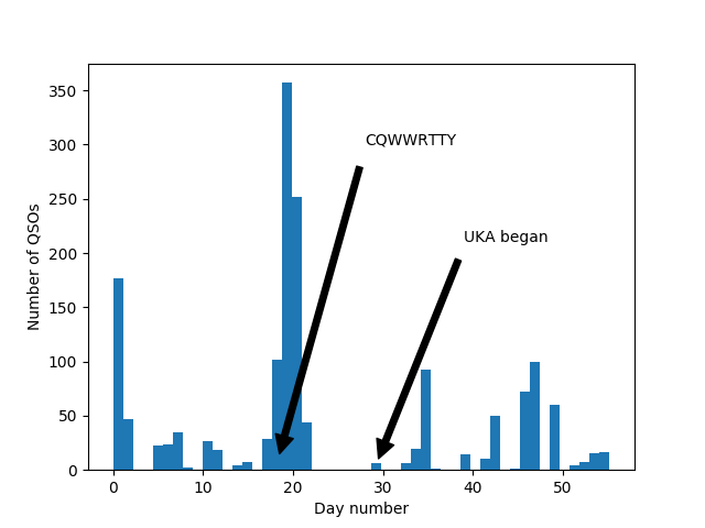
The number of QSOs distributed across the days since we started using the callsign. The general level of activity is more or less equal before and after the start of UKA, with the most activity occurring during CQWWRTTY and a burst of activity at the very beginning.

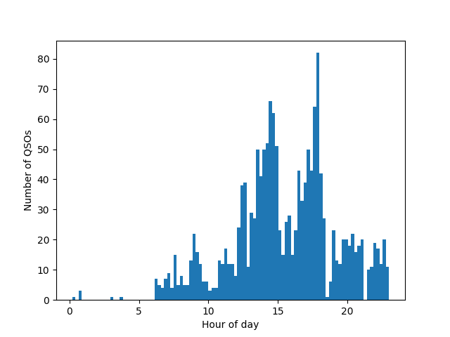
The number of QSOs as a function of hour during the day (UTC). This distribution follows more or less what is expected from the distribution of people at ARK, with a post-work/post-study day frenzy at around 16.00 NT and after 18.00 NT (UTC time had an offset of -2 hours from Norwegian time during UKA).

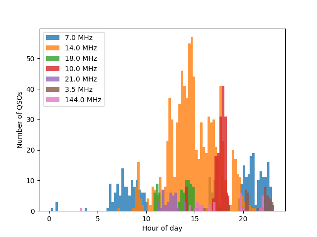
The same plot as above, but split on the used band. “Day” and “night” bands (14.0 MHz and 7.0 MHz, respectively) can clearly be seen, along with spurious use of e.g. 10.0 MHz during the afternoon.

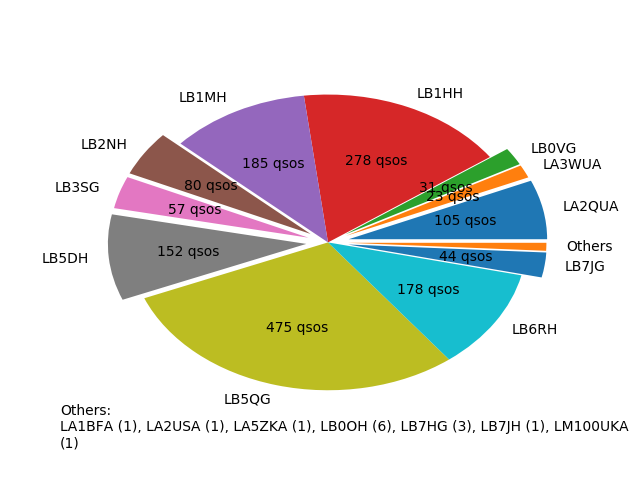
The distribution of QSOs among the various operators.

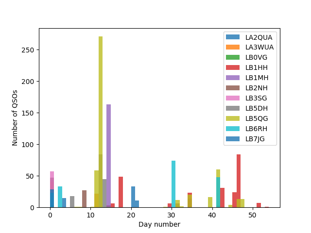
The distribution of operators during the building period and UKA itself. A variety of operators participated during the building period, while the start of UKA itself posed some difficulties in both avoiding  interference and being able to get into Samfundet due to stricter access regimes. Mainly LB5QG and  LB1HH kept going during this last phase.

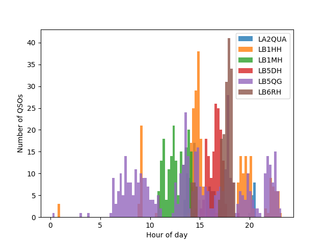
The distribution of operators during the hours of the day. LB5QG has done a considerable effort in producing QSOs at all hours of the day.

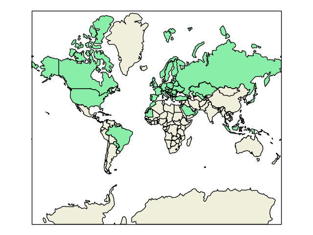
World map with filled countries corresponding to the countries we have run. This also involved reading of a HTML table from the ITU website into a Pandas dataframe in order to convert from callsign prefix to country, made easy by pandas.read_html(..) :-). Here, we could also technically have used the ClubLog API to look up country information from the callsigns, but would probably put a bit of a strain on the servers if we were to do that for all calls in the log. Instead, we hacked together a solution using the official ITU allocation tables.

The script used in generating the above plots can be found at github. This is made to analyze all .s3db-files in a folder, and differs a bit from the code snipped shown in the beginning of this post.

Only our most recent, still-in-use logs are in .s3db-format, however, as we strive to convert to ADIF format or similar during the archival process. We’ll also look into what we can extract from the larger bulk of older logs.