Sampling at high sample rates from an SDR in GNU Radio with slow blocks in the flowgraph (for example writing to file on a slow hard drive) can lead to missing samples. In this blog post, we give a complete method for rectifying for the missing samples during off-line analysis so that the samples appear to be timed.
During one of the blog posts dealing with antenna pattern extraction from measurements of our beacons at Vassfjellet, we had an interesting situation in that post-processing of measurements of LA2VHF produced perfectly timed morse sequences, while measurements of LA2SHF produced sequences that were significantly offset from each other. The question was whether LA2SHF produced inconsistent morse code, or whether there was something wrong with our measurement setup. LA2SHF was measured at 1 MHz, while LA2VHF was measured at 0.1 MHz, which should have been a major clue to what was the problem :-).
Sampling at a high sample rate might cause overflow errors, which means that the host computer can’t process the incoming samples at the rate they are delivered, which again means that the USRP has to drop samples. This is usually detected by the handling software, and is notified to the user by printing subtle “O” to standard output. The author didn’t look for those, however, especially since overflow wasn’t expected for sample rates at 1 MHz. Due to the uncertainty, the author therefore had to go back and measure both beacons at different sample rates in order to completely leave out the possibility that LA2SHF had timing problems in its morse code, and that this was just overflows and timing errors during our reception chain.
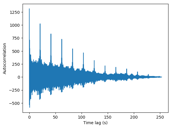
The beacons were measured for 120 seconds, which was hoped to cover enough sequences of the repeated signal to see the timing offsets in the autocorrelation. Extracting the sequence periods from the autocorrelation of the sampled data confirmed that the timing offsets were in place only for sample rates of 1 MHz:
| samp_rate | frequency | sequence_periods | period_diff |
|---|---|---|---|
| 100000.0 | 1296963000 | [2006, 2006, 2006, 2006, 2006] | 0 |
| 100000.0 | 144463000 | [3028, 3028, 3028] | 0 |
| 1000000.0 | 1296963000 | [20060, 19808, 20057, 20061, 20060] | 253 |
| 1000000.0 | 144463000 | [30279, 30277, 30279] | 2 |
(The sequence periods are measured in number of samples, and are the distance from peak to peak in the autocorrelation diagram, the difference is calculated from the maximum and minimum of the derived sequence periods. The sequence periods are expected to be equal when there are no timing problems.)
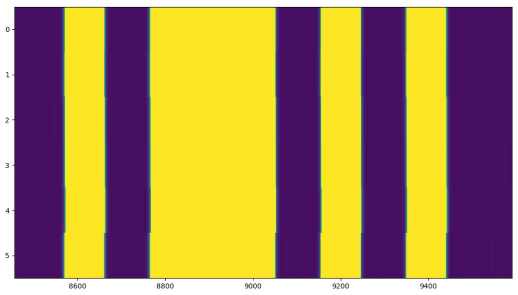
The offsets are higher for LA2SHF than LA2VHF in this case, but this is mainly because 120 seconds allows for 5 sequences from LA2SHF, and only 3 sequences for LA2VHF, which is due to the sequences being longer for LA2VHF:
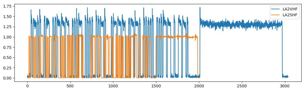
Above are sequences from LA2SHF and LA2VHF measured for the same sample rate and FFT length, meaning that each sample in the sequences corresponds to the same timestep. Interestingly, LA2SHF has been set up to transmit a faster morse signal than LA2VHF. Since a measurement with a given length of LA2SHF has room for more sequences, the sequence extraction becomes more sensitive to timing offsets, as more sequences have to match perfectly. For LA2VHF, we only have to match 2-3 sequences. Offsets in one sequence matched against another sequence might cancel each other out, but won’t cancel for a sequence matched against four other sequences.
That the timing problem is due to overflows is also very evident by the fact that the GNU Radio flowgraph printed “OOO” during the reception of this measurement series, indicating at least three overflows, which we’d noticed if we had followed the standard output of GNU Radio companion more diligently during the pattern measurements. This is not very interesting, and is a known problem that should be accounted for by ensuring that the computer is up to speed, the blocks can handle the stream, the connection to the USRP is fast enough and so on. This is mainly us having made a mistake. The interesting part is how to rectify for these measurement errors if such overflows are unavoidable, or we have acquired data with overflows and can’t or don’t want to repeat the measurements, and have to make do with what we have.
We assume during loading of the GNU Radio samples that the samples are produced at a regular rate, and that timestamps for each sample can be calculated from the timestamp of the first sample and the sample rate. During overflow this is no longer true. There are two options here: Either, samples are always associated with individual timestamps, and the timestamps are rectified where there is overflow, or samples can be added to rectify for the missing samples. Always having to carry around timestamps with samples at irregular intervals quickly gets inconvenient since much of the processing methods assume regular sampling. It is therefore probably better to fill the missing samples so that the timestamps are regular, and that we only need timestamps of first and last sample to fully specify the time axis of the measurement.
Either way, we need to know when the overflows happen. Luckily, this behavior is fully specified and present in the GNU Radio meta file sink data. The UHD manual specifies that ‘O’ is printed to stdout when an overflow is detected, as observed, and that it “pushes an inline message packet into the receive stream“. GNU Radio therefore gets a message whenever an overflow occurs. The GNU Radio API manual for the USRP source specifies that a new timestamp is produced whenever an overflow occurs, which is probably triggered by the UHD message, and therefore our main indication of overflows. All tags are recorded by the GNU Radio file meta file sink, so that we actually can use this information to rectify for timing problems in the signal.
The GNU Radio meta file sink produces a header and data, as explained in a previous blog post. The header has multiple elements. The code here reads the first header element, which fully specifies all we usually need to know (like center frequency, sample rate, first timestamp, …). There is another header element after that, which is read by moving the file pointer to the end of the first header element and reading the next as if it was the first. Header elements are organized as a long string of header elements:
[ header 1 | header 2 | ... | header N-1 | header N]
The first header element consists of the following elements:
{'nitems': 1000,
 'hdr_len': 171,
 'cplx': True,
 'rx_rate': 99999.99968834173,
 'nbytes': 8000,
 'extra_len': 22,
 'has_extra': True,
 'rx_freq': 1.29694e+09,
 'type': 'float',
 'rx_time': 1532034082.183634,
 'size': 8}
Most of the header elements are the same as the first. The very last header element has a few fields changed:
'nitems': 456,
'nbytes': 3648,
'rx_time': 1532034202.2436345,
nbytes and nitems probably controls how many elements the header properties apply to, and the number is changed for the last element because the GNU Radio flowgraph was stopped at an arbitrary time, and not exactly when a multiple of 1000 samples had been collected. rx_time is the timestamp, and is mainly the only field that changes from header element to header element. rx_rate is also unchanged regardless of overflows.
Given no overflow, the difference in rx_time from header element to header element should be constant and correspond to the sample rate multiplied by the number of samples represented by the header. Calculating the difference between subsequent timestamps shows clearly where there were overflows:
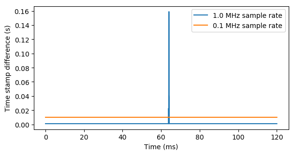
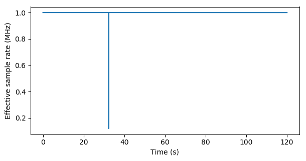
The time stamp differences can also be used to calculate effective sample rates.
There is one gotcha here, however, as new timestamp tag also might be issued when frequency or gain settings are changed. It is important to rectify the time stamp differences against the number of items for which the timestamp change is valid. This rectification does not result in a very large difference in the above plots, but the numerical difference is important for subsequent analysis.
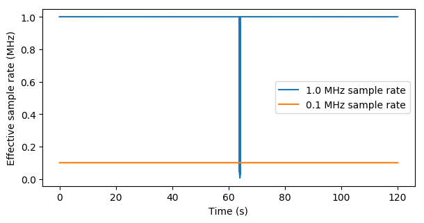
Zooming in on the problematic area 64 seconds into the measurement shows four large deviations, but also that the effective sample rate is unstable for all samples:

The measurement at 0.1 MHz also has some small deviations in the effective sample rate, but not as extensive as for the 1 MHz sample rate.

There are therefore symptoms of starting overflow problems at both sample rates, not always resulting in an actual overflow. This is a bit unexpected, as the computer should be able to handle the data stream rate, even at 1 MHz. But: We are using a file sink… The file sink works against a hard drive and does file IO, which is extremely slow and jittery compared to the fast processes happening on the CPU and in the RAM, and especially compared to the high sample rates of the data arriving from the USRP. The GNU Radio file meta sink continuously writes to the specified files, and is at the mercy of the speed of the file operations. Some buffering will happen against the hard drive, and the GNU Radio flowgraph will also buffer up samples when it sees that some blocks are slower than the others, but the buffers have limits. Especially for high sample rates producing file sizes in the order of gigabytes.
One similar, major overflow also happens during the LA2VHF measurement at 1 MHz, but at a different position in time, and with less spikes. The behavior is not very predictable, and would be subject to other file IO operations happening on the system.
The hope is that the issued time stamps can be used to rectify the measurement. One problem might be that since the overflow happened due to a buffer overflow problem, the missed samples will not directly correspond to the sample position at which we have the derived rate change, but this will probably just cause random errors and not a systematic error.
We investigated timestamps and number of items for a range of header elements describing an obvious overflow problem. (Timestamps are taken relative to the first element in the range, since writing out the full nanosecond UNIX timestamp gets a bit cumbersome).
| element | timestamps | num_items | delta_time |
|---|---|---|---|
| (ms) | (ms) | ||
| 1 | 0.000 | 1000 | – |
| 2 | 1.000 | 1000 | 1.000 |
| 3 | 2.000 | 747 | 1.000 |
| 4 | 24.66 | 1000 | 22.66 |
| 5 | 25.66 | 1000 | 1.000 |
Notice that the timestep discrepancy happens from the third to fourth element, but that the number of items changes only for the third element. When the overflow occurred above, the count over a “packet” of 1000 items is aborted and stopped at 747 items, and a new count is started for the next packet, which then starts at a new timestamp. The discrepancy in the number of items is mainly due to the flowgraph having to issue a new timestamp immediately after the overflow, so that the preceding packet had to have less than 1000 items. The “missing” number of items in the num_items column therefore has nothing to do with the actual missing samples, this is only a book-keeping convenience.
The actual number of missing samples is the number of samples we normally would expect during a time span of 22.66 milliseconds with a constant sample rate, and not 1000-747. The samples are missing from element 3 to element 4. Deviations in the delta_time column from the expected sample period therefore applies to the previous row. This could be an important distinction, as we’d rather not associate the timing problem with the wrong set of samples and get off-by-one errors.
Given one of the normal elements with 1000 items, the sample rate of 1000 kHz yields an expected delta_time of 1/(1000 kHz) * 1000 items = 1 ms, as seen above. The element with 747 samples should on the other hand have generated a delta_time of 1/(1000 kHz) * 747 = 0.747 ms. The measured time difference of 22.66 ms minus this figure should therefore yield the total time passed with missing samples, which again can give us the actual number of missing samples at this element by multiplying with the expected sample rate. The number of missing samples here is 23 913.59. (We’ll come back to the decimal.)
The expected number of samples can be calculated as expected_samples = f_s * np.diff(timestamps). The missing samples can be calculated as missing_samples = expected_samples - num_items. Indices each header element correspond to can be found by sample_counter = np.cumsum(num_items).astype(int).
Problem indices are detected by finding indices where missing_samples is larger than zero. IQ samples are copied out unmodified in-between the problem indices, while exactly at the problem indices are new, interpolated IQ-samples mass-produced to match the number of missing samples.
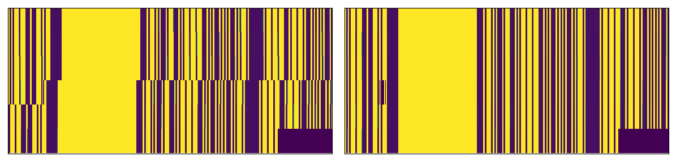
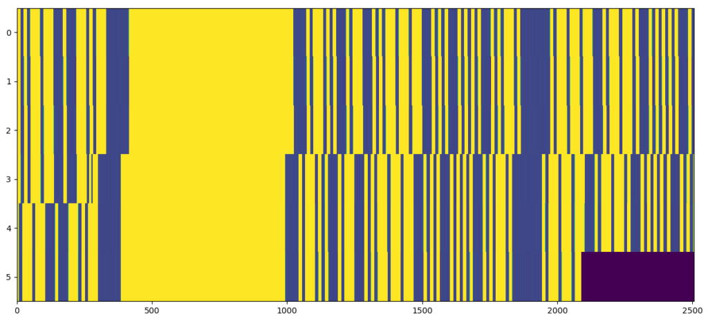
The end result for this approach is not that bad:
Before rectification, showing obvious timing offsets:
After rectification:
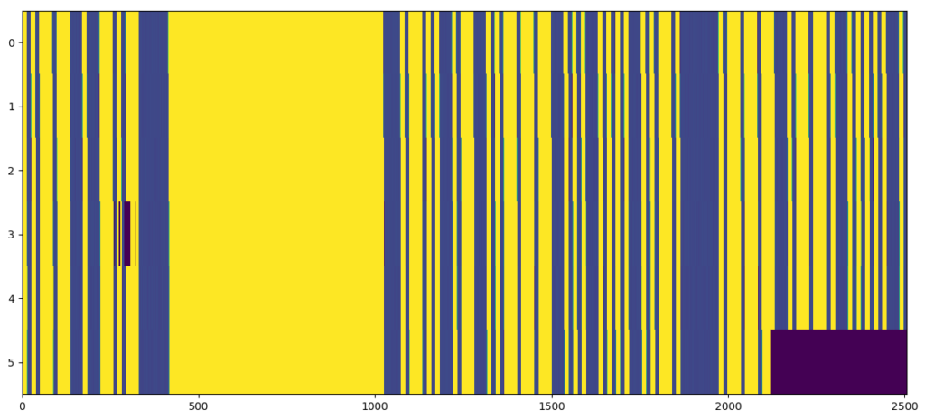
Obviously, the filled samples don’t have correct values (appears as black boxes in the sequence diagram), but the timing offsets are not longer horrible. Filling with NaN or something could be used to rectify for the timing, but make us able to ignore these samples during processing. If we look very closely at the signals, it can be seen that there still are some very small offsets:

Above, we converted missing_samples to integers. They are actually floating point numbers:
-0.0725 -0.0725 0.1700 -0.0725 -0.0725
It was seen above that the effective sample rate was noisy even outside of the overflow areas. No samples are missed here, the samples are just not received with precise timing due to the same reasons we end up with overflow errors in the first place, and the imprecise timing is quantified by a missing sample count going up and down. The missing samples above adds up to something close to 0 in the long run, meaning that this effect leads to a consistent number of samples, and that we can’t rectify for it by adding samples. Technically, it could be rectified by removing or adding samples to the packets and keeping strict control over the sample inventory count, but this gets tricky. It would also lead to more useless samples that interfere with the subsequent processing. An elaborate interpolation scheme could also be applied to correct for the timing.
Crosscorrelation on each sequence as used in Extracting the antenna pattern from a beacon signal, pt. II: Measurements of LA2SHF leads to the following:
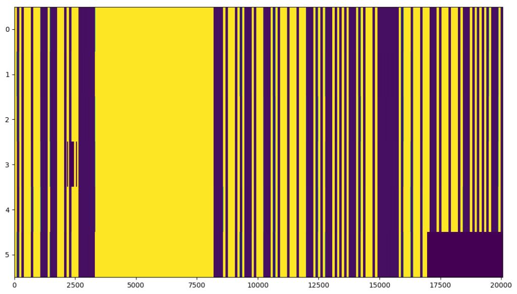
Some deviations are still seen, as the deviations will occur randomly throughout a single sequence. Still, we’re far better off now than we were without the overflow correction in the beginning.
The rectification code is available on GitHub. Unfortunately, it isn’t appropriate to insert the missing samples or interpolate during preprocessing. The file sizes are high at the high sample rates, and it is necessary to use memory mapping to avoid loading the entire files in memory. The processing in our case involves extracting specific FFT bins, which is less memory intensive, but having to insert artificial missing samples require that the full file is loaded into memory before any other processing is applied. The overflow rectification is therefore done as an conversion operation on the file itself, to be written to another GNU Radio file.
The corrections done here might not always be desirable since they insert artificial samples into the data, but the presented methods gives some basic tools for extracting the real timestamps of each packet of samples. This can be used to deal with the problem also in other ways.

0 Comments
1 Pingback