We have published a couple of posts ([1], [2], [3]) on how to measure an antenna pattern by using an external signal source, which we successfully used to debug our parabolic dish. The signal source measured was a constant carrier wave, which makes it easier to calculate the antenna pattern, since we just have to measure the signal at varying azimuth degrees. The main focus was to get a measurement quickly to be able to debug and fix the antenna setup.
It could be useful to characterize our antennas at any time against the beacons we have installed at Vassfjellet mountain. This could be used to quickly evaluate the antenna performance if we suspect there is something wrong with it (for example useful in Thermal cycling and the woes of the northern amateur during the suspicion stage). This requires a simple procedure for antenna diagram evaluation. If we want to be able to automatically calibrate our antenna rotors against said beacons, antenna diagrams would also be valuable.
In general, the signal to be measured is usually not a carrier wave. Our beacons at Vassfjellet send out a morse signal, along with a long BEEEEEP!, but measuring exactly at the BEEEEEEP! is a long and tedious process we’d rather avoid. Rapidly sweeping over all azimuth angles while measuring the morse signal, and not caring about dihs and dahs would be the least tedious process. Post-processing could handle the extraction of the enveloping variation in signal level around the morse signal.
The main problem is to determine what is an actual low signal level, and what is just the beacon signal being stopped. Here is an illustration of the problem through an actual measurement of the LA2VHF beacon while rotating the antenna:
![]()
The first part (approx. until 12 seconds into the measurement) is with the parabola pointing towards -90 degrees azimuth, and is rather stable. A simple threshold would be sufficient here to extract the underlying morse signal, and interpolate the signal level.
Once the antenna starts rotating, the signal level varies dramatically, however. A simple threshold would remove also lower signal levels, and remove valuable information on the pattern.
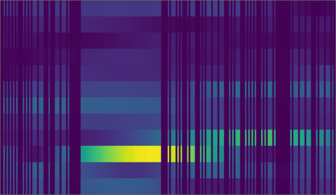
Plotting the full measurement series for a full turn shows how the antenna pattern clearly modulates the morse signal:
![]()
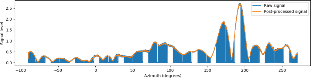
Or with azimuth angles along the x-axis instead of seconds, as interpolated using our previously presented Python software package:
![]()
For visual inspection of the pattern, this is actually enough and we could stop here. The pattern is visible enough for us humans to judge the lobe and take coherent decisions.
Plotting this in a polar diagram would be extremely ugly due to the signal level rapidly going up and down, however. It also gets harder to subject the pattern to further analysis. Having this many data points to plot or analyze is also a waste of memory, as the pattern can be represented using a sparser set of points, but this is difficult to express without having extracted the enveloping signal level modulation. Taking the mean or trying to interpolate directly will discard a lot of information or transform the pattern. We’d therefore rather, of course, continue on to extracting the modulated signal level and take the gaps in the signal as an extra, exciting challenge.
What I originally wanted to do was to apply a more probabilistic approach by attempting to characterize the background signal level and try to segment out the beacon signal by comparing level distributions. This does kind of neglect the fact that the signal here is very deterministic, however :-). It is a regular morse signal being turned off and off by a machine, timed and perfect. LB6RH Jens suggested to use a correlation-based scheme to extract the timings.
The first approach was to correlate the signal against a square pulse with varying lengths. This shows how the morse signal is composed of a dih, dah and a BEEEEEEEEEEEEEEEP, with lengths 7, 27 and 484 samples, respectively, indicated by peaks in the correlation diagrams for the respective lengths.

Technically, the correlation analysis could extract all the dihs, dahs and the BEEEEEEEEEEEEEEEEP! directly, but it gets a bit difficult to extract the information programmatically, especially when the signal level varies. The approach could be improved or made more advanced, but a simpler and more powerful technique would be to just use autocorrelation.
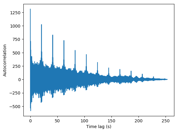
Autocorrelation means that the signal is correlated with a lagged copy of itself. A large autocorrelation value at a specific lag T means that the signal repeats itself or looks a lot like itself after T timesteps. A signal which is deterministic and repeats itself regularly – like ours – should have a very clear autocorrelation pattern. Any signal which repeats itself to some extent usually have a lot of information in the autocorrelation diagram (music, heartbeats, …), and our signal is even better.

This plot is symmetric about the y-axis, so the autcorrelation is shown only for positive time lags. There are prominent, thin peaks in place, which should be an indication of where the morse signal sequence is repeated throughout the measurement. There is also a vague triangular baseline in the plot, which suggests that there is a “DC-component” in the signal which dominates over the smaller variations in which we are interested. The slowly varying DC-component should be removed to yield a signal which is centered around the x-axis.
Technically, this DC-component behavior is actually the modulation which is due to change in azimuth angle. Ironically, to get a good autocorrelation so that we can extract this, we need to have already extracted it so that we can calculate the autocorrelation to extract it. We’ll therefore settle for an approximation by taking the central moving average to be a rough estimate of the enveloping behavior. If there was no enveloping behavior, we could have subtracted the DC component/constant/bias by subtracing the mean.
![]()
Subtracting the central moving average from the signal should yield a signal with less DC component, and therefore an autocorrelation with less triangular behavior:
Success! We now have more clear peaks. Zooming into the first three peaks shows the following:

The peaks are easy to see. Extracting them is a bit more challenging, since the other parts of the autocorrelation also are spiky and have peak-like behaviors. The variations here are mostly due to noise, but it might also be possible to extract information about the individual timings of the morse signal from it. We’ll settle with the main peaks for now, however. The first peaks are marked below:

The difference in between each peak is exactly 2020 samples, or 20.685 seconds. These peaks indicate when the morse sequence is repeated, and the difference should correspond to the length of the repeated sequence. We can confirm this by marking the morse sequence with stops calculated from the sequence length found above.
![]()
This exercise mainly shows us that the signal is periodic, and what the period is, in terms of the discretization of the measured data. The actual morse sequence starts somewhere after the long BEEEEP!, while “our” sequence here starts when we start the measurement. This doesn’t matter, since the sequence is periodic in any case.
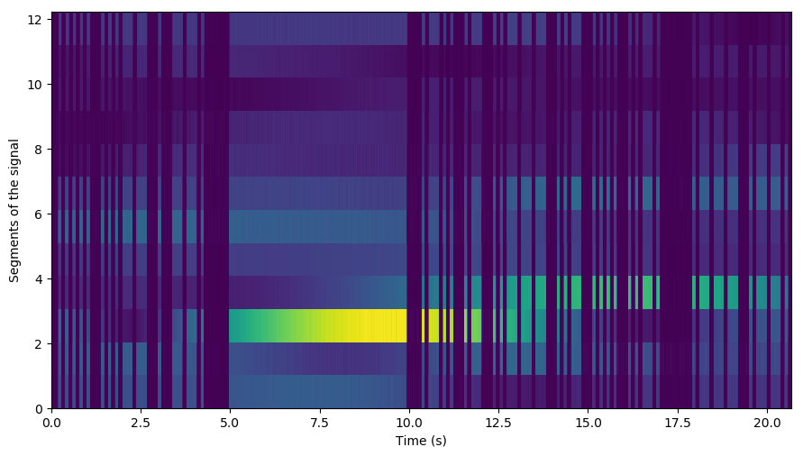
We can then separate the full measurement into its constituent morse sequences, and see how the morse sequence repeats itself, only modulated by the change in the azimuth angle:
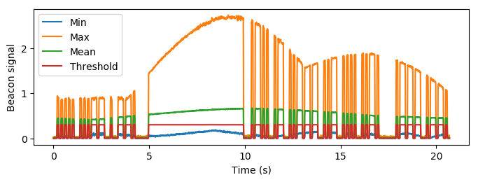
We now know the position of each sequence exacly. The task now is to interpolate the gaps throughout the entire measurement series. Taking the min, max and mean across sequences produces the following:
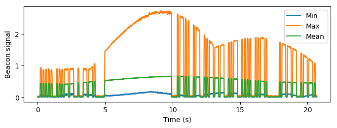
Even at the lowest signal level, there is a semi-clear morse sequence. By combining all sequences, we have enough data to threshold the data and get out how the sequence actually behaves. We constructed the threshold here based on the mean of the mean value, which feels a bit fishy and ad-hoc and I don’t really like doing things like this, but at least the threshold is not arbitrary.
If the threshold is chosen from the mean value and the maximum value is the one thresholded, it can also be argued that it won’t miss any samples. If the signal level is very low throughout the entire signal, we could have that some samples would be dominated by noise and a maximum which is thresholded incorrectly, but I doubt that there would be any pattern to extract in any case if that was the case.
![]()
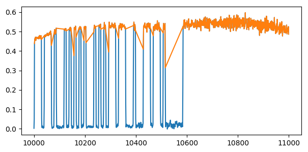
Overlapping the extracted morse sequence with the measured, modulated signal shows a perfect match. We’re almost there, and could almost use this to extract the signal level.
One remaining problem is that some samples are taken as the beacon signal rises from the background level to the signal level, and are counted (correctly) as a part of the morse signal.
This has to do with the time resolution, and that some parts of the signal always will be captured exactly when it has risen, while other samples will be calculated during the rise time, or that the FFT produces values trapped between background and signal level (probably more likely). The autocorrelation will still find the correct signal frames, but the thresholded signal will sometimes include rising samples which does not look that good when what we want is the underlying modulation pattern.
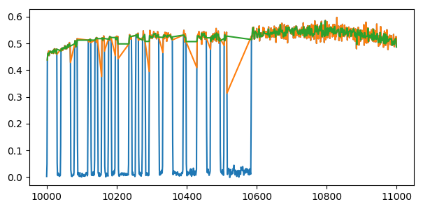
This would mostly seem to happen with single samples at the edges, and is a type of noise which is easily removed by applying a median filter (green):
Those lines over each gap (linear interpolation) look ugly due to the the modulating level having noise added on top of it, so we’ll have to apply better interpolation. Some kind of spline interpolation with a sufficient smoothing factor is probably what would be the most suitable:

But! Linear interpolation does not look that bad when we consider the entire pattern :-).
Linear interpolation is also faster, while spline interpolation can be a bit slow when this many datapoints are used, or at least it was slow with the type of spline I used. Some more work could be done here for optimality.
There are a couple of problems with the approach outlined in this blog post:
- We were extremely lucky with the time resolution of the samples. This does not usually happen using the approach in this blog post, as the signal sequence will start and stop at arbitrary times, but our time resolution can cause each signal segment to be e.g. 2025.3333333333 samples, instead of exactly 2020 samples. This causes a systematic offset, and the approach will be vulnerable to this as we assume exact timing during post-processing.
- We measured LA2VHF (2m wavelength) on an antenna made for 23 cm wavelengths. The pattern seen above is actually very bad, which makes the processing simpler, as the beacon signal itself is not that dominated by the pattern behavior. For signals that are optimal for the antenna in use, the main lobe corresponding to the direction of the signal source could be 30-40 dB higher than the surrounding lobes. This will cause the lobe pattern to dominate over the individual morse samples in the autocorrelation, and will show how the lobes are correlated against each other, and not the morse sequence.
Since ARK mostly is dormant due to the summer vacation, there is not much activity going on. In order to have enough to write blog posts about through the entire summer, we’ll divide this small subproject into three more posts:
- A blog post about a more robust approach as developed and tested for LA2SHF.
- A blog post outlining the code used for frequency analysis and the complete, more robust method for extraction of the enveloping signal.
- Investigations into a more probabilistic approach, and comparison against the deterministic approach that is implicitly used here. Initial tests I did when trying to construct an overengineered GNU Radio module for pattern analysis showed some promising results using this approach, but I predict that it will fail for the lower signal levels. It is probably interesting in any case, and a nice repetition on hypothesis testing from your basic Statistics course.
Or this is at least the plan. Stay tuned! More to come. LA3WUA Øyvind also has some nice hand held radio tests lined up which will be published throughout the summer.
Next parts in the complete series:
- Extracting the antenna pattern from a beacon signal, pt. I: Initial investigations using autocorrelation (current post)
- Extracting the antenna pattern from a beacon signal, pt. II: Measurements of LA2SHF
- Extracting the antenna pattern from a beacon signal, pt. III: Frequency analysis and code
- Extracting the antenna pattern from a beacon signal, pt. IV: Probabilistic approach

0 Comments
4 Pingbacks